Perform alternative splicing analysis for multiple Visium samples

On this page

• 0. Prepare the data.
• 1. Preprocess all four slices and intergrate them into one object
• 2. Visualize genome tracks of multiple samples
• Optional: Build cell-cell weight matrix by spatial coordinates

This vignette demonstrates how to analyze alternative splicing across multiple Visium samples. The procedure for spatial transcriptomics follows the same principles as scRNA-seq but requires careful handling of imaging data and spatial coordinates for accurate visualization. Additionally, this example illustrates how to visualize genome tracks from multiple BAM files.

0. Prepare the data.

We will use four Visium slices for 10X data source page. These slices come from two sections, each section contain two slices, one is sagittal anterior, and another one is sagittal posterior of mouse brain. We download the processed BAM files, and annotated them with PISA.

Section 1, sagittal anterior

Section 1, sagittal posterior

Section 2, sagittal anterior

Section 2, sagittal posterior

The following commands run on a terminal.

# Create directory for each section and slice
mkdir -p visium/section1/Posterior
mkdir -p visium/section1/Anterior
mkdir -p visium/section2/Posterior
mkdir -p visium/section2/Anterior

# Enter to work directory and download GTF for mouse
cd visium;
wget -c https://ftp.ebi.ac.uk/pub/databases/gencode/Gencode_mouse/release_M10/gencode.vM10.annotation.gtf.gz

# Download the bam file and image files to each directory
cd section1/Posterior
wget -c https://cf.10xgenomics.com/samples/spatial-exp/1.1.0/V1_Mouse_Brain_Sagittal_Posterior/V1_Mouse_Brain_Sagittal_Posterior_possorted_genome_bam.bam
wget -c https://cf.10xgenomics.com/samples/spatial-exp/1.1.0/V1_Mouse_Brain_Sagittal_Posterior/V1_Mouse_Brain_Sagittal_Posterior_possorted_genome_bam.bam.bai
wget -c https://cf.10xgenomics.com/samples/spatial-exp/1.1.0/V1_Mouse_Brain_Sagittal_Posterior/V1_Mouse_Brain_Sagittal_Posterior_spatial.tar.gz

# unpack image files
tar zxvf V1_Mouse_Brain_Sagittal_Posterior_spatial.tar.gz

# Annotate and count features
PISA anno -gtf ../../gencode.vM10.annotation.gtf.gz -exon -psi -o anno.bam -t 7 V1_Mouse_Brain_Sagittal_Posterior_possorted_genome_bam.bam

mkdir exp
mkdir exon
mkdir junction
mkdir exclude
PISA count -tag CB -umi UB -anno-tag GN -outdir exp anno.bam
PISA count -tag CB -umi UB -anno-tag EX -outdir exon anno.bam
PISA count -tag CB -umi UB -anno-tag JC -outdir junction anno.bam
PISA count -tag CB -umi UB -anno-tag ER -outdir exclude anno.bam

## Go back to work directory, and reenter to another slice's directory
cd -; 
cd section1/Anterior
wget -c https://s3-us-west-2.amazonaws.com/10x.files/samples/spatial-exp/1.1.0/V1_Mouse_Brain_Sagittal_Anterior/V1_Mouse_Brain_Sagittal_Anterior_possorted_genome_bam.bam
wget -c https://cf.10xgenomics.com/samples/spatial-exp/1.1.0/V1_Mouse_Brain_Sagittal_Anterior/V1_Mouse_Brain_Sagittal_Anterior_possorted_genome_bam.bam.bai
wget -c https://cf.10xgenomics.com/samples/spatial-exp/1.1.0/V1_Mouse_Brain_Sagittal_Anterior/V1_Mouse_Brain_Sagittal_Anterior_spatial.tar.gz

# unpack image file
tar zxvf V1_Mouse_Brain_Sagittal_Anterior_spatial.tar.gz

# Annotate and count features
PISA anno -gtf ../../gencode.vM10.annotation.gtf.gz -exon -psi -o anno.bam -t 7 V1_Mouse_Brain_Sagittal_Anterior_possorted_genome_bam.bam

mkdir exp
mkdir exon
mkdir junction
mkdir exclude
PISA count -tag CB -umi UB -anno-tag GN -outdir exp anno.bam
PISA count -tag CB -umi UB -anno-tag EX -outdir exon anno.bam
PISA count -tag CB -umi UB -anno-tag JC -outdir junction anno.bam
PISA count -tag CB -umi UB -anno-tag ER -outdir exclude anno.bam

# Swith to section 2 
cd -;
cd section2/Anterior
wget -c https://s3-us-west-2.amazonaws.com/10x.files/samples/spatial-exp/1.1.0/V1_Mouse_Brain_Sagittal_Anterior_Section_2/V1_Mouse_Brain_Sagittal_Anterior_Section_2_possorted_genome_bam.bam
wget -c https://cf.10xgenomics.com/samples/spatial-exp/1.1.0/V1_Mouse_Brain_Sagittal_Anterior_Section_2/V1_Mouse_Brain_Sagittal_Anterior_Section_2_possorted_genome_bam.bam.bai
wget -c https://cf.10xgenomics.com/samples/spatial-exp/1.1.0/V1_Mouse_Brain_Sagittal_Anterior_Section_2/V1_Mouse_Brain_Sagittal_Anterior_Section_2_spatial.tar.gz

tar zxvf V1_Mouse_Brain_Sagittal_Anterior_Section_2_spatial.tar.gz

PISA anno -gtf ../../gencode.vM10.annotation.gtf.gz -exon -psi -o anno.bam -t 7 V1_Mouse_Brain_Sagittal_Anterior_Section_2_possorted_genome_bam.bam

mkdir exp
mkdir exon
mkdir junction
mkdir exclude
PISA count -tag CB -umi UB -anno-tag GN -outdir exp anno.bam
PISA count -tag CB -umi UB -anno-tag EX -outdir exon anno.bam
PISA count -tag CB -umi UB -anno-tag JC -outdir junction anno.bam
PISA count -tag CB -umi UB -anno-tag ER -outdir exclude anno.bam


cd -;
cd section2/Sagittal
wget -c https://cf.10xgenomics.com/samples/spatial-exp/1.1.0/V1_Mouse_Brain_Sagittal_Posterior_Section_2/V1_Mouse_Brain_Sagittal_Posterior_Section_2_possorted_genome_bam.bam
wget -c https://cf.10xgenomics.com/samples/spatial-exp/1.1.0/V1_Mouse_Brain_Sagittal_Posterior_Section_2/V1_Mouse_Brain_Sagittal_Posterior_Section_2_possorted_genome_bam.bam.bai
wget -c https://cf.10xgenomics.com/samples/spatial-exp/1.1.0/V1_Mouse_Brain_Sagittal_Posterior_Section_2/V1_Mouse_Brain_Sagittal_Posterior_Section_2_spatial.tar.gz

tar zxvf V1_Mouse_Brain_Sagittal_Posterior_Section_2_spatial.tar.gz

PISA anno -gtf ../../gencode.vM10.annotation.gtf.gz -exon -psi -o anno.bam -t 7 V1_Mouse_Brain_Sagittal_Posterior_Section_2_possorted_genome_bam.bam

mkdir exp
mkdir exon
mkdir junction
mkdir exclude
PISA count -tag CB -umi UB -anno-tag GN -outdir exp anno.bam
PISA count -tag CB -umi UB -anno-tag EX -outdir exon anno.bam
PISA count -tag CB -umi UB -anno-tag JC -outdir junction anno.bam
PISA count -tag CB -umi UB -anno-tag ER -outdir exclude anno.bam

# Now go back to work directory
cd ../../..

1. Preprocess all four slices and intergrate them into one object

This section will perform Seurat pipeline for all the sections. A Seurat workflow for one section can be found here https://satijalab.org/seurat/articles/spatial_vignette. The difference between this workflow with Seurat’s is we use counts generated from PISA, while Seurat use counts generated with CellRanger’s pipeline. For the details of different between PISA and CellRanger, please see our manual.

require(Seurat)

Loading required package: Seurat

Loading required package: SeuratObject

Loading required package: sp

Attaching package: 'SeuratObject'

The following objects are masked from 'package:base':

    intersect, t

require(dplyr)

Loading required package: dplyr

Attaching package: 'dplyr'

The following objects are masked from 'package:stats':

    filter, lag

The following objects are masked from 'package:base':

    intersect, setdiff, setequal, union

require(Yano)

Loading required package: Yano

exp.1 <- ReadPISA("./visium/section1/Anterior/exp/", prefix = "sec1_ant_")
image.1 <- Read10X_Image("./visium/section1/Anterior/spatial/")
new.names <- paste0("sec1_ant_",Cells(image.1))
image.1 <- RenameCells(image.1, new.names = new.names)

## QuickRecipe() is actually an integration function of Seurat workflow
obj.1 <- QuickRecipe(exp.1[, Cells(image.1)], verbose = FALSE)
obj.1[['slice1']] <- image.1[colnames(obj.1),]
obj.1$orig.ident <- "sec1_ant"

exp.2 <- ReadPISA("./visium/section1/Posterior/exp/", prefix = "sec1_pos_")
image.2 <- Read10X_Image("./visium/section1/Posterior/spatial/")
new.names <- paste0("sec1_pos_",Cells(image.2))
image.2 <- RenameCells(image.2, new.names = new.names)
obj.2 <- QuickRecipe(exp.2[,Cells(image.2)], verbose = FALSE)
obj.2[['slice2']] <- image.2[colnames(obj.2),]
obj.2$orig.ident <- "sec1_pos"

exp.3 <- ReadPISA("./visium/section2/Anterior/exp/", prefix="sec2_ant_")
image.3 <- Read10X_Image("./visium/section2/Anterior/spatial/")
new.names <- paste0("sec2_ant_",Cells(image.3))
image.3 <- RenameCells(image.3, new.names = new.names)
obj.3 <- QuickRecipe(exp.3[, Cells(image.3)], verbose = FALSE)
obj.3[['slice3']] <- image.3[colnames(obj.3),]
obj.3$orig.ident <- "sec2_ant"

exp.4 <- ReadPISA("./visium/section2/Posterior/exp/", prefix="sec2_pos_")
image.4 <- Read10X_Image("./visium/section2/Posterior/spatial/")
new.names <- paste0("sec2_pos_",Cells(image.4))
image.4 <- RenameCells(image.4, new.names = new.names)
obj.4 <- QuickRecipe(exp.4[, Cells(image.4)], verbose = FALSE)
obj.4[['slice4']] <- image.4[colnames(obj.4),]
obj.4$orig.ident <- "sec2_pos"

# Merge all processed Seurat object
obj <- merge(obj.1, y = list(obj.2, obj.3, obj.4))

obj <- QuickRecipe(obj)

Set default assay to RNA

object <- NormalizeData(object, normalization.method = "LogNormalize", scale.factor = 10000)

Normalizing layer: counts.1

Normalizing layer: counts.2

Normalizing layer: counts.3

Normalizing layer: counts.4

object <- FindVariableFeatures(object, selection.method = "vst", nfeatures = 3000)

Finding variable features for layer counts.1

Finding variable features for layer counts.2

Finding variable features for layer counts.3

Finding variable features for layer counts.4

object <- ScaleData(object, features =  @features)

Centering and scaling data matrix

object <- RunPCA(object, features = @features

PC_ 1 
Positive:  Trf, Apod, Plekhb1, Mbp, Cnp, Plp1, Mobp, Car2, Mag, Dbi 
       Cryab, Mog, Cldn11, Bcas1, Sept4, Mal, Ndrg1, Ptgds, Gatm, Ermn 
       Qdpr, Ppp1r14a, Sparc, Gsn, Ugt8a, Gfap, Fa2h, Gm20425, Pllp, Tmem88b 
Negative:  Calm2, Ctxn1, Rtn1, Chn1, Nrgn, Syt1, Ppp3r1, Cx3cl1, Ptprn, Gria2 
       Gpm6a, Sept5, Ptk2b, Gp1bb, Enc1, Calm1, Fbxl16, Basp1, Arf3, Snca 
       Meg3, Camkv, Hpcal4, Syt5, Chst1, Nsg2, Icam5, Ppp3ca, Pld3, Dclk1 
PC_ 2 
Positive:  Tmsb4x, Nrgn, Inf2, Ctxn1, Ngef, Gpr88, Gng7, Ddn, Adcy5, Pde1b 
       Camkv, Rgs9, Phactr1, Kcnip2, Klhl2, Ptk2b, Lrrc10b, Ptpn5, Tac1, Cx3cl1 
       Adora2a, Bcl11b, Efnb3, Crip2, Mal, Pde2a, Ppp1r1a, Tmem158, Basp1, Hpca 
Negative:  Cbln1, Car8, Neurod1, Pcp2, Gm2694, Ppp1r17, Lhx1os, Zic1, Nrep, Shf 
       Rgs8, Kcnc3, Grin2c, Ank1, Inpp5a, Homer3, Grm4, Pvalb, Kcnc1, Il16 
       Sphkap, Icmt, Calb2, Trim62, Gng13, Il20rb, Chn2, Pagr1a, Dusp5, Atp2a3 
PC_ 3 
Positive:  Cck, Stmn1, Gnas, Nrn1, 3110035E14Rik, Slc17a7, Olfm1, Vsnl1, Tbr1, Lingo1 
       Stx1a, Slc30a3, Ncald, Dkk3, Efhd2, Rtn4r, Neurod6, Miat, 1110008P14Rik, Gm11549 
       Mpped1, Basp1, Pde1a, Gabbr2, Nsmf, Fxyd7, Syt13, Mical2, E130012A19Rik, Osbpl1a 
Negative:  Penk, Rgs9, Adora2a, Pde10a, Ppp1r1b, Gpr88, Drd1, Syndig1l, Gpr6, Tac1 
       Lrrc10b, Rxrg, Adcy5, Scn4b, Pde1b, Rasd2, Gng7, Rarb, Slc35d3, Tmem158 
       Actn2, Serpina9, Strip2, Slc32a1, Ankrd63, Kcnab1, Dmkn, Gnal, Pcp4l1, St8sia3 
PC_ 4 
Positive:  Scn4b, Mbp, Slc24a2, Qdpr, Mobp, Mag, Bcas1, Nefm, Plp1, Mal 
       Plekhb1, Vamp1, Nefl, Sept4, Ermn, Tspan2, Mog, Arpp19, Trf, Cnp 
       Cryab, AI593442, Pex5l, Tmem88b, Gpr37, Ppp1r14a, Pllp, Uchl1, Kcnab1, Snap25 
Negative:  Igf2, Islr, Igfbp2, Slc13a4, Mgp, Fmod, Slc6a20a, Aebp1, Ogn, Nnat 
       Slc6a13, Col1a2, Fabp7, Aldh1a2, Rbp1, Gjb2, Pcolce, Slc22a6, Slc13a3, Bmp7 
       Dcn, Fn1, Serping1, Col1a1, Crabp2, Ifitm3, Efemp1, Bgn, Vim, Fbln1 
PC_ 5 
Positive:  Itpr1, Itpka, Zbtb18, Cplx2, Adcy1, Rnf112, Nptx1, Lmo4, Hpca, Neurod2 
       Dkk3, Sptbn2, Camk4, Cnr1, Cnksr2, Arpp19, Fbxl16, Tmem132a, Igf2, Prkcb 
       Atp1a1, Dgkz, Lzts3, Mmp17, Ppp1r1b, Neurl1a, Slc8a2, Gas7, Slc13a4, Fam212b 
Negative:  Slc6a11, Gng4, Nrip3, Scg2, Ptpro, Sp8, Dlx1, Hap1, Cdhr1, Th 
       Doc2g, Zcchc12, Pcbp3, Pbx3, Scgn, Dcx, Tshz1, Tuba1a, A230065H16Rik, Tubb3 
       Cacng5, Pcp4l1, Cpne4, Lgr5, Lgr6, Sp9, Dlx2, Tmem130, Adamts19, Tubb2a 

object <- FindNeighbors(object, dims = 1:20)

Computing nearest neighbor graph

Computing SNN

object <- FindClusters(object, resolution = 0.5)

Modularity Optimizer version 1.3.0 by Ludo Waltman and Nees Jan van Eck

Number of nodes: 12148
Number of edges: 388028

Running Louvain algorithm...
Maximum modularity in 10 random starts: 0.9315
Number of communities: 16
Elapsed time: 0 seconds

object <- RunUMAP(object, dims = 1:20)

14:46:37 UMAP embedding parameters a = 0.9922 b = 1.112

14:46:37 Read 12148 rows and found 20 numeric columns

14:46:37 Using Annoy for neighbor search, n_neighbors = 30

14:46:37 Building Annoy index with metric = cosine, n_trees = 50

0%   10   20   30   40   50   60   70   80   90   100%

[----|----|----|----|----|----|----|----|----|----|

**************************************************|
14:46:42 Writing NN index file to temp file /local/tmp/RtmpWPaWRY/file21c4cb60805922
14:46:42 Searching Annoy index using 1 thread, search_k = 3000
14:47:01 Annoy recall = 100%
14:47:01 Commencing smooth kNN distance calibration using 1 thread with target n_neighbors = 30
14:47:02 Initializing from normalized Laplacian + noise (using RSpectra)
14:47:16 Commencing optimization for 200 epochs, with 500526 positive edges
14:47:16 Using rng type: pcg
14:47:31 Optimization finished

p1 <- DimPlot(obj, group.by = "orig.ident")
p2 <- DimPlot(obj)
p1 + p2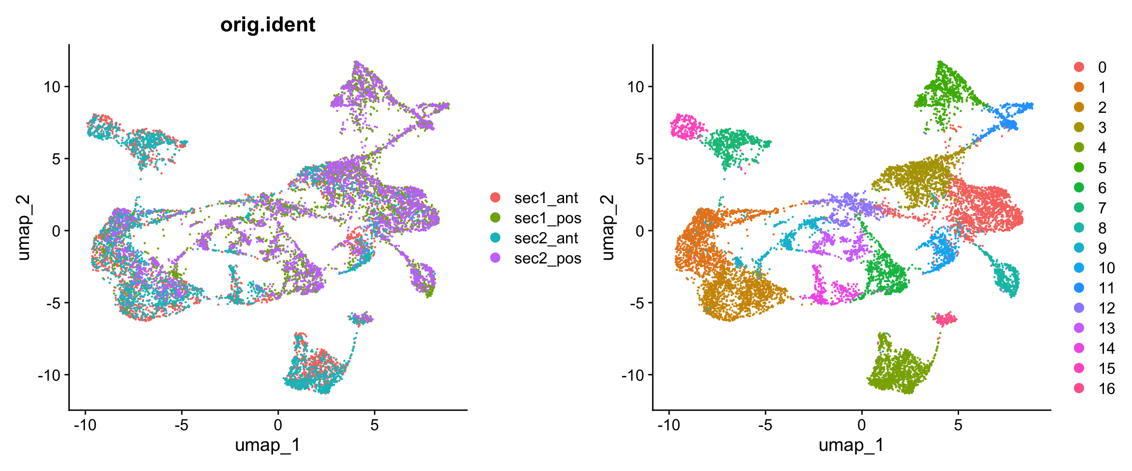

SpatialPlot(obj, pt.size.factor = 2)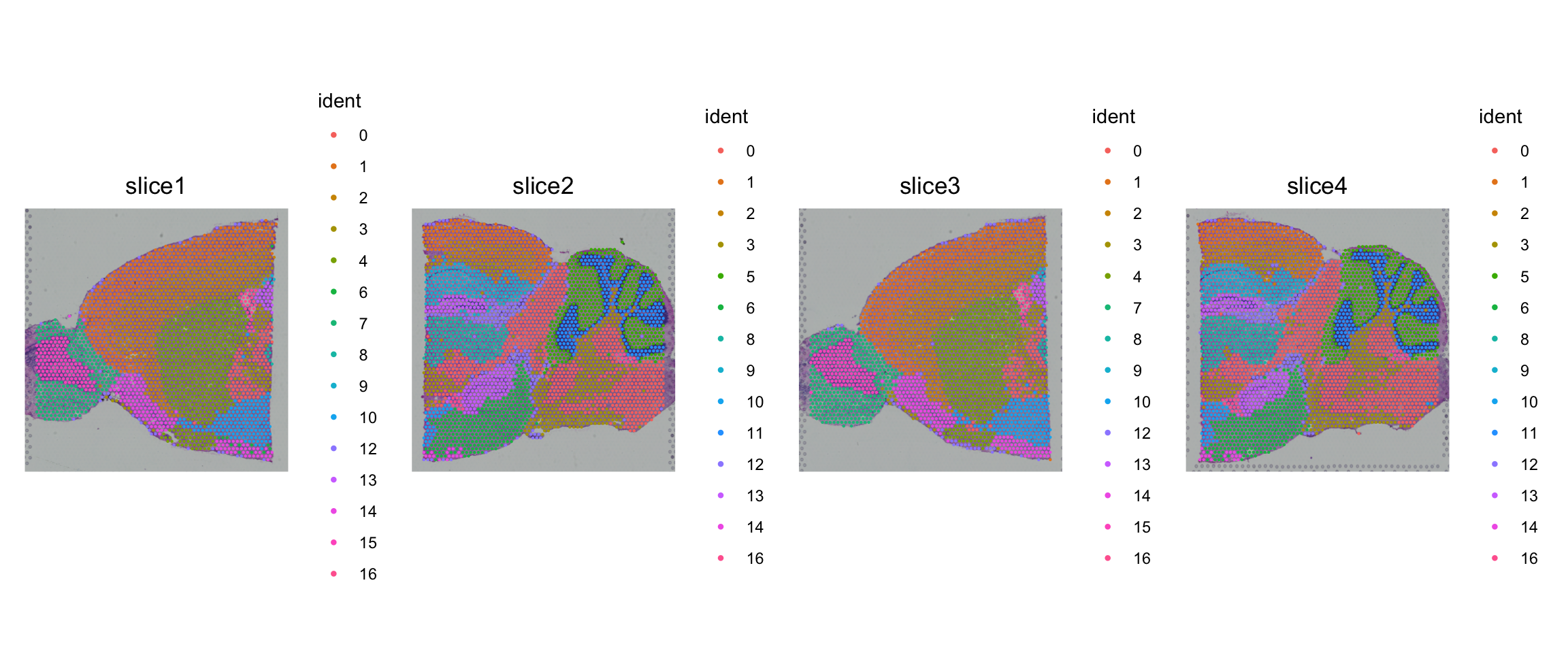 

exon.1 <- ReadPISA("./visium/section1/Anterior/exon/", prefix = "sec1_ant_", cells = Cells(obj))
exon.2 <- ReadPISA("./visium/section1/Posterior/exon/", prefix = "sec1_pos_", cells = Cells(obj))
exon.3 <- ReadPISA("./visium/section2/Anterior/exon/", prefix = "sec2_ant_", cells = Cells(obj))
exon.4 <- ReadPISA("./visium/section2/Posterior/exon/", prefix = "sec2_pos_", cells = Cells(obj))
exon <- mergeMatrix(exon.1, exon.2, exon.3, exon.4)

'as(<dgTMatrix>, "dgCMatrix")' is deprecated.
Use 'as(., "CsparseMatrix")' instead.
See help("Deprecated") and help("Matrix-deprecated").

obj[['exon']] <- CreateAssayObject(exon[, Cells(obj)], min.cells = 20)
DefaultAssay(obj) <- "exon"
obj <- NormalizeData(obj)
obj <- ParseExonName(obj)

Working on assay exon

obj <- RunAutoCorr(obj)

Working on assay : exon
Run autocorrelation test for 80178 features.
Runtime : 20.818 secs
38784 autocorrelated features.

obj <- RunSDT(obj, bind.name = "gene_name", bind.assay = "RNA")

Working on assay exon.
Working on binding assay RNA.
Use predefined weight matrix "pca_wm".
Processing 38784 features.
Processing 15696 binding features.
Retrieve binding data from assay RNA.
Use "data" layer for test features and binding features.
Using 95 threads.
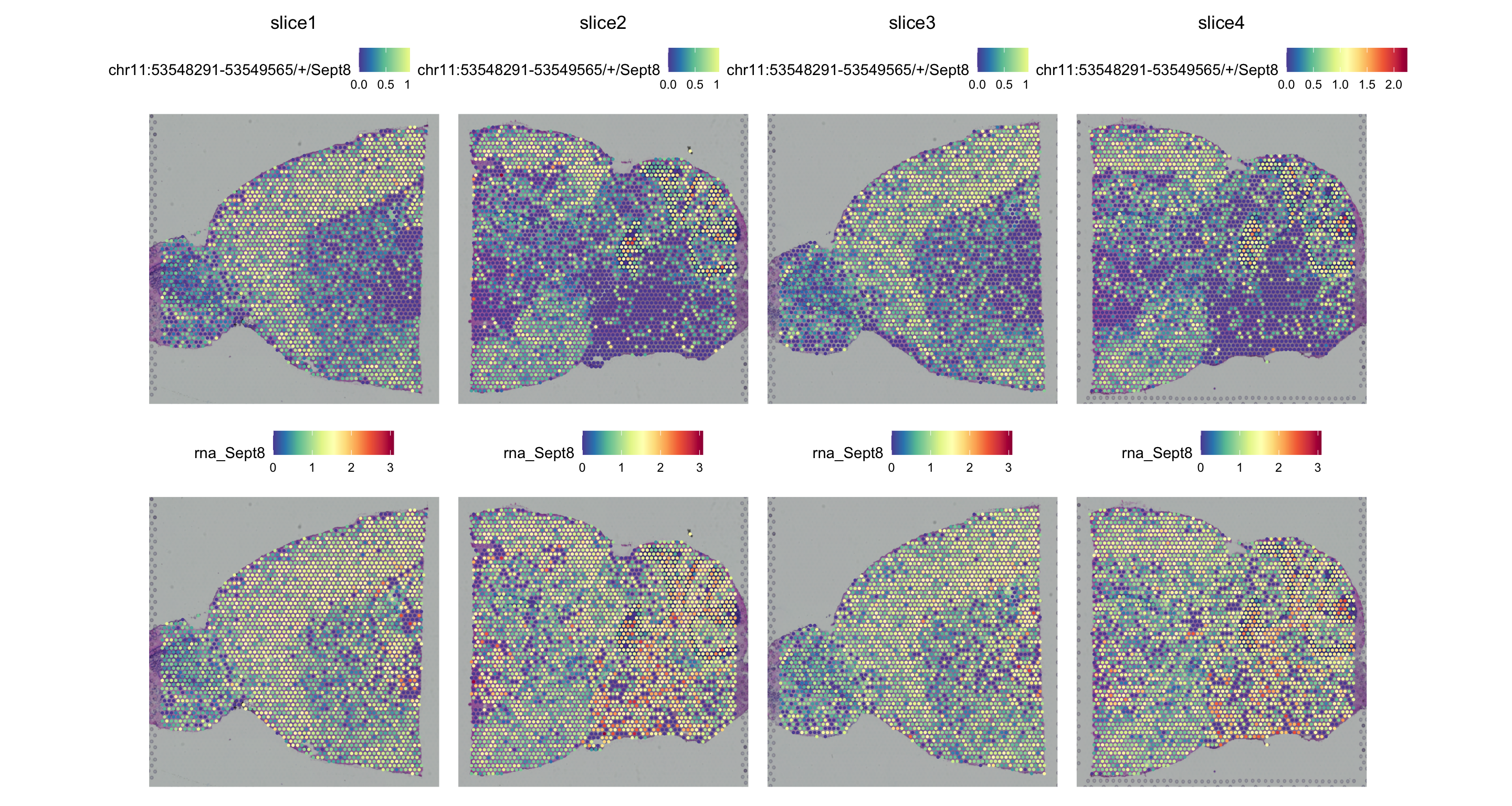
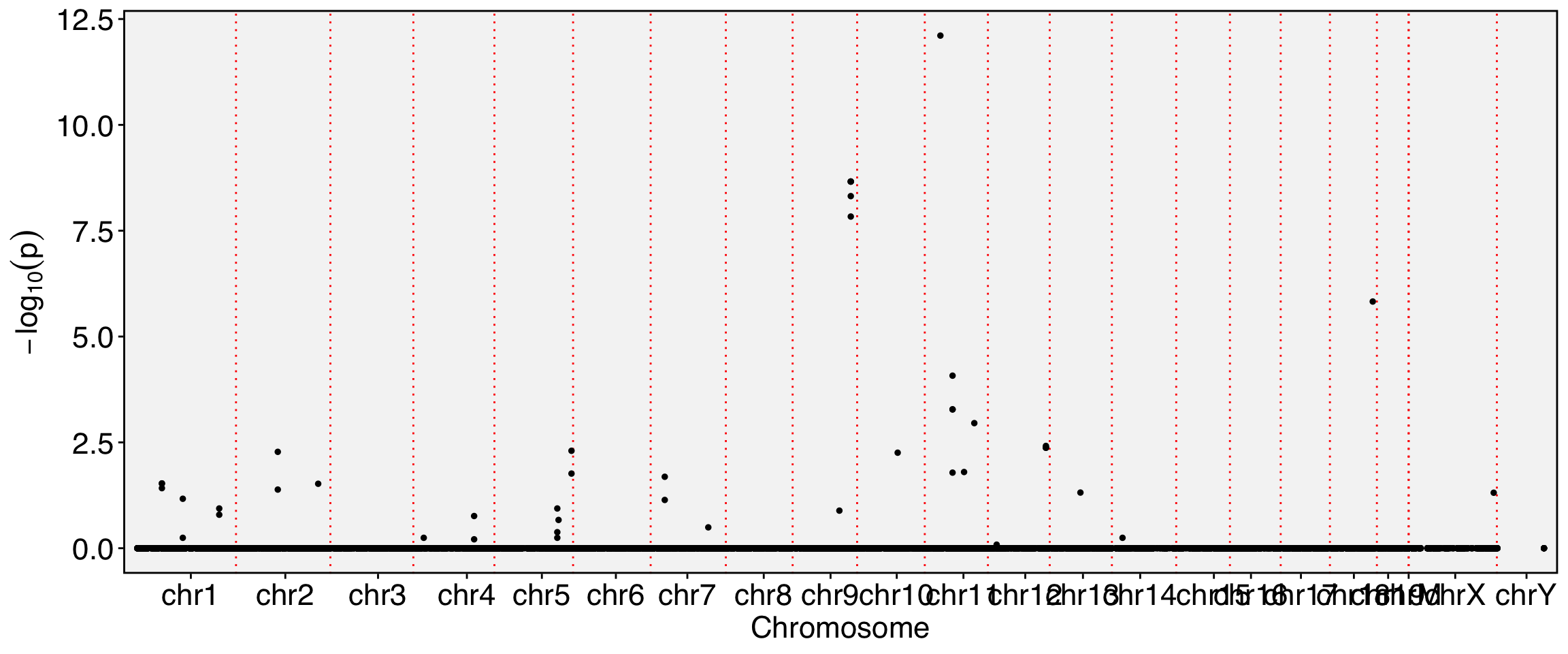
Runtime : 2.730924 mins.

FbtPlot(obj, val = "gene_name.padj")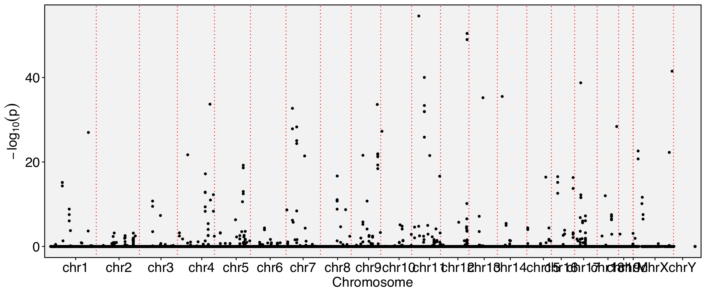

obj[['exon']][[]] %>% filter(gene_name.padj<1e-10) %>% DT::datatable()

SpatialPlot(obj, features = c("chr11:53548291-53549565/+/Sept8","Sept8"), pt.size.factor = 2)

2. Visualize genome tracks of multiple samples

Since the spot/cell names have already been renamed in the Seurat object, we need to define a binding list that maps the new cell names to their original names, which will be used for reading sequences from the BAM files. In this vignette, we use four BAM files, requiring us to define four corresponding cell vectors. Each vector contains group factor values, where the names of the values correspond to the original cell names in the BAM file.

gtf <- gtf2db("./visium/gencode.vM10.annotation.gtf.gz")

[2026-06-15 14:52:36] GTF loading..
[2026-06-15 14:52:51] Load 48440 genes.
[2026-06-15 14:52:51] Load time : 14.983 sec

bamfiles <- list(
  sec1_ant = "./visium/section1/Anterior/V1_Mouse_Brain_Sagittal_Anterior_possorted_genome_bam.bam",
  sec1_pos = "./visium/section1/Posterior/V1_Mouse_Brain_Sagittal_Posterior_possorted_genome_bam.bam",
  sec2_ant = "./visium/section2/Anterior/V1_Mouse_Brain_Sagittal_Anterior_Section_2_possorted_genome_bam.bam",
  sec2_pos = "./visium/section2/Posterior/V1_Mouse_Brain_Sagittal_Posterior_Section_2_possorted_genome_bam.bam"
  )

cell.list <- split(obj$seurat_clusters, obj$orig.ident)
str(cell.list)

List of 4
 $ sec1_ant: Factor w/ 16 levels "0","1","2","3",..: 10 10 10 5 5 5 5 10 5 10 ...
  ..- attr(*, "names")= chr [1:2695] "sec1_ant_TTGCCGGTGATCCCTC-1" "sec1_ant_CGGTATAGGTATTAGC-1" "sec1_ant_CGTTGAGTAATTGCGT-1" "sec1_ant_TAAATGCCGTCTCATG-1" ...
 $ sec1_pos: Factor w/ 16 levels "0","1","2","3",..: 10 10 10 10 10 10 10 10 10 10 ...
  ..- attr(*, "names")= chr [1:3342] "sec1_pos_TGGGACCATTGGGAGT-1" "sec1_pos_CCGGTGCGAGTGATAG-1" "sec1_pos_TAGCCAGAGGGTCCGG-1" "sec1_pos_GAAGGGCATAACCATG-1" ...
 $ sec2_ant: Factor w/ 16 levels "0","1","2","3",..: 10 10 10 10 10 10 10 10 10 5 ...
  ..- attr(*, "names")= chr [1:2823] "sec2_ant_TTGAGGCATTTAACTC-1" "sec2_ant_CACCGGAGATATCTCC-1" "sec2_ant_CACGTCTATGATGTGG-1" "sec2_ant_TGACCAGCTTCAAAGT-1" ...
 $ sec2_pos: Factor w/ 16 levels "0","1","2","3",..: 10 10 10 10 10 10 10 10 10 10 ...
  ..- attr(*, "names")= chr [1:3288] "sec2_pos_TCCGCAGCCACCTAGC-1" "sec2_pos_GGTCCTTCATACGACT-1" "sec2_pos_GTGCCTAGCTATGCTT-1" "sec2_pos_GCGAGAAACGGGAGTT-1" ...

cell.list1 <- lapply(cell.list, function(x) {
  nm <- names(x)
  names(x) <- gsub(".*_(.*)","\\1",nm)
  x
})
str(cell.list1)

List of 4
 $ sec1_ant: Factor w/ 16 levels "0","1","2","3",..: 10 10 10 5 5 5 5 10 5 10 ...
  ..- attr(*, "names")= chr [1:2695] "TTGCCGGTGATCCCTC-1" "CGGTATAGGTATTAGC-1" "CGTTGAGTAATTGCGT-1" "TAAATGCCGTCTCATG-1" ...
 $ sec1_pos: Factor w/ 16 levels "0","1","2","3",..: 10 10 10 10 10 10 10 10 10 10 ...
  ..- attr(*, "names")= chr [1:3342] "TGGGACCATTGGGAGT-1" "CCGGTGCGAGTGATAG-1" "TAGCCAGAGGGTCCGG-1" "GAAGGGCATAACCATG-1" ...
 $ sec2_ant: Factor w/ 16 levels "0","1","2","3",..: 10 10 10 10 10 10 10 10 10 5 ...
  ..- attr(*, "names")= chr [1:2823] "TTGAGGCATTTAACTC-1" "CACCGGAGATATCTCC-1" "CACGTCTATGATGTGG-1" "TGACCAGCTTCAAAGT-1" ...
 $ sec2_pos: Factor w/ 16 levels "0","1","2","3",..: 10 10 10 10 10 10 10 10 10 10 ...
  ..- attr(*, "names")= chr [1:3288] "TCCGCAGCCACCTAGC-1" "GGTCCTTCATACGACT-1" "GTGCCTAGCTATGCTT-1" "GCGAGAAACGGGAGTT-1" ...

TrackPlot(bamfile = bamfiles, cell.group = cell.list1, gtf = gtf, gene = "Sept8", highlights = c(53548291,53549565), junc=TRUE)

Optional: Build cell-cell weight matrix by spatial coordinates

We previously used PCA to construct the cell weight matrix, but for spatial transcriptomics data, it is also possible to use the spatial coordinates, the real spot-to-spot distances, to build the weight matrix. Here, we demonstrate how to do this.

Starting from Yano v1.4, Yano supports building the weight matrix from multiple slices simultaneously. When multiple image names are passed to RunAutoCorr(), GetWeightsFromSpatial() computes the spatial weight matrix for each image individually and then merges them into a single combined weight matrix via mergeMatrix(). This allows the spatial correlation analysis to leverage all slices together without needing to subset or analyze each slice separately.

# Use spatial coordinates from all four slices
obj <- RunAutoCorr(obj, image = c("slice1", "slice2", "slice3", "slice4"))

Working on assay : exon

Run autocorrelation test for 80178 features.

Runtime : 37.547 secs

36013 autocorrelated features.

grep("_wm", names(obj), value=TRUE)

[1] "pca_wm"     "spatial_wm"

obj <- RunSDT(obj, bind.name = "gene_name", bind.assay = "RNA", wm.name = "spatial_wm")

Working on assay exon.

Working on binding assay RNA.

Use predefined weight matrix "spatial_wm".

Processing 36013 features.

Processing 14739 binding features.

Retrieve binding data from assay RNA.

Use "data" layer for test features and binding features.

Using 95 threads.

Runtime : 1.973901 mins.

FbtPlot(obj, val = "gene_name.padj")

Meta(obj) %>% filter(gene_name.padj<1e-10) %>% DT::datatable()

# SpatialFeaturePlot can display the results on any individual slice
SpatialFeaturePlot(obj, features = c("chr11:30106785-30109152/-/Sptbn1","Sptbn1"), images = c("slice1", "slice2", "slice3", "slice4"))