On this page
This vignette demonstrates how to use Yano buildin functions to interactively select or pick cells/spots from a plot using your mouse and keyboard. While tools like CellxGene are widely used for this purpose, to the best of our knowledge, an efficient solution for performing this task within the R environment is still lacking. Here, we introduce a lightweight, fast and native implementation of a cell selector to address this gap.
Prepare the data.
We use demo data from SeuratData for simplity.
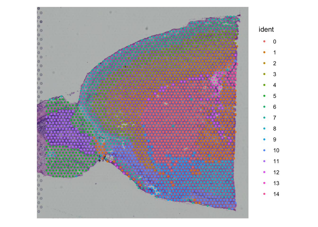
require (Yano)require (Seurat)require (SeuratData)InstallData ("stxBrain" )<- LoadData ("stxBrain" , type = "anterior1" )<- SCTransform (brain, assay = "Spatial" , verbose = FALSE )<- RunPCA (brain, assay = "SCT" , verbose = FALSE )<- FindNeighbors (brain, reduction = "pca" , dims = 1 : 30 )<- FindClusters (brain, verbose = FALSE )<- RunUMAP (brain, reduction = "pca" , dims = 1 : 30 )SpatialPlot (brain)
Select spots from spatial plot
.1 <- SpatialSelector (brain)Press ESC on your keyboard to exist the selection!
Now the selected cells will be exported to sel.1. If you want return a object, try to set return.object=TRUE in the function.
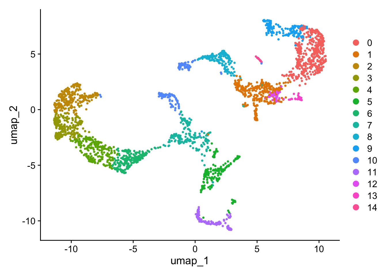
Select cells from dimension reduction plot
We can also select cells from dimension reduction plot.
.1 <- DimSelector (brain)Press ESC on your keyboard to exist the selection!
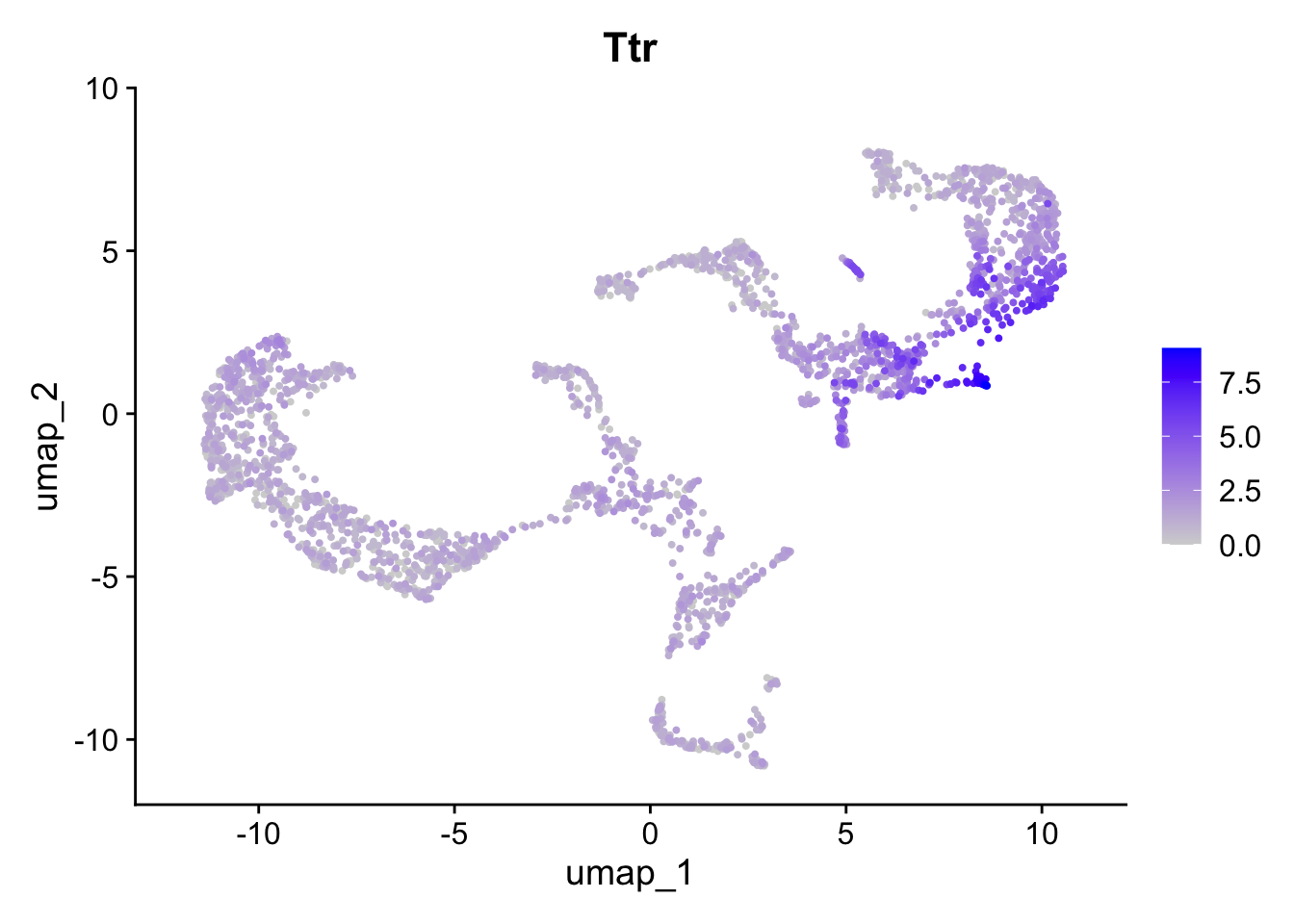
Select cells based on a feature expression
FeaturePlot (brain, features = c ('Ttr' ), order= TRUE )
FeatureSelector (brain, feature = c ('Ttr' ), order= TRUE )Please note in FeatureSelector() only one feature is support at each selection. Therefore, I designed the parameter feature instead of orignal features here.
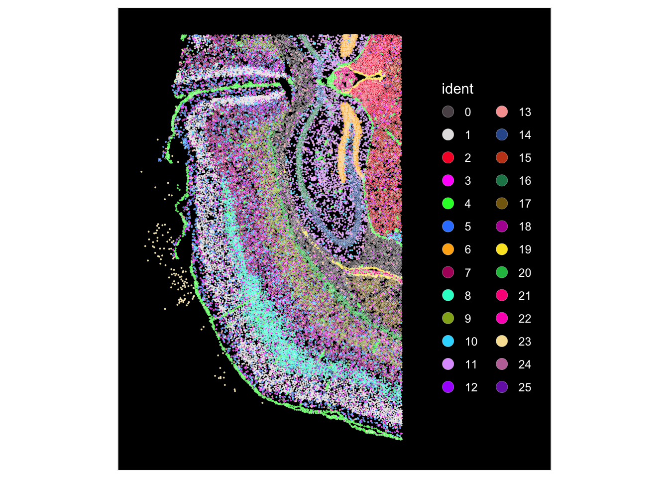
Select cells from Image-based spatial data
Here we will use 10x Genomics Xenium data, generated from Seurat’s tutorial .
<- readRDS ("xenium.rds" )ImageDimPlot (xenium.obj, border.color = "white" , border.size = 0.1 , cols = "polychrome" )
Warning: No FOV associated with assay 'SCT', using global default FOV
ImageDimSelector (xenium.obj, border.color = "white" , border.size = 0.1 )
Generate 2D concave hull of selected region
In spatial transcriptomics, it is sometimes necessary to manually define capsule or membrane regions, as these areas are often thin, mixed with neighboring cells, and difficult to identify accurately. Manually specifying these regions can be beneficial for downstream analyses, where precise spatial organization of cells is critical for understanding tissue architecture and functional gradients.
<- SpatialConcaveHull (brain)
Questions?
If you have any questions regarding this vignette, the usage of Yano or suggestions, please feel free to report them through the discussion forum .
R version 4.5.3 (2026-03-11)
Platform: x86_64-pc-linux-gnu
Running under: Ubuntu 24.04.4 LTS

Matrix products: default
BLAS:   /usr/lib/x86_64-linux-gnu/openblas-pthread/libblas.so.3
LAPACK: /usr/lib/x86_64-linux-gnu/openblas-pthread/libopenblasp-r0.3.26.so;  LAPACK version 3.12.0

locale:
 [1] LC_CTYPE=C.UTF-8       LC_NUMERIC=C           LC_TIME=C.UTF-8
 [4] LC_COLLATE=C.UTF-8     LC_MONETARY=C.UTF-8    LC_MESSAGES=C.UTF-8
 [7] LC_PAPER=C.UTF-8       LC_NAME=C              LC_ADDRESS=C
[10] LC_TELEPHONE=C         LC_MEASUREMENT=C.UTF-8 LC_IDENTIFICATION=C

time zone: Etc/UTC
tzcode source: system (glibc)

attached base packages:
[1] stats     graphics  grDevices utils     datasets  methods   base

other attached packages:
[1] future_1.70.0             stxBrain.SeuratData_0.1.2
[3] SeuratData_0.2.2.9002     Seurat_5.4.0
[5] SeuratObject_5.3.0        sp_2.2-1
[7] Yano_1.5

loaded via a namespace (and not attached):
  [1] RColorBrewer_1.1-3          jsonlite_2.0.0
  [3] magrittr_2.0.4              spatstat.utils_3.2-2
  [5] farver_2.1.2                rmarkdown_2.30
  [7] vctrs_0.7.2                 ROCR_1.0-12
  [9] DelayedMatrixStats_1.30.0   spatstat.explore_3.8-0
 [11] S4Arrays_1.8.1              htmltools_0.5.9
 [13] SparseArray_1.8.1           sctransform_0.4.3
 [15] parallelly_1.46.1           KernSmooth_2.23-26
 [17] htmlwidgets_1.6.4           ica_1.0-3
 [19] plyr_1.8.9                  plotly_4.12.0
 [21] zoo_1.8-15                  igraph_2.2.2
 [23] mime_0.13                   lifecycle_1.0.5
 [25] pkgconfig_2.0.3             Matrix_1.7-5
 [27] R6_2.6.1                    fastmap_1.2.0
 [29] GenomeInfoDbData_1.2.14     MatrixGenerics_1.22.0
 [31] fitdistrplus_1.2-6          shiny_1.13.0
 [33] digest_0.6.39               patchwork_1.3.2
 [35] S4Vectors_0.48.1            tensor_1.5.1
 [37] RSpectra_0.16-2             irlba_2.3.7
 [39] GenomicRanges_1.60.0        beachmat_2.26.0
 [41] labeling_0.4.3              progressr_0.18.0
 [43] spatstat.sparse_3.1-0       httr_1.4.8
 [45] polyclip_1.10-7             abind_1.4-8
 [47] compiler_4.5.3              withr_3.0.2
 [49] S7_0.2.1                    viridis_0.6.5
 [51] fastDummies_1.7.5           MASS_7.3-65
 [53] DelayedArray_0.34.1         rappdirs_0.3.4
 [55] gtools_3.9.5                tools_4.5.3
 [57] lmtest_0.9-40               otel_0.2.0
 [59] httpuv_1.6.17               future.apply_1.20.2
 [61] goftest_1.2-3               glmGamPoi_1.20.0
 [63] glue_1.8.0                  nlme_3.1-168
 [65] promises_1.5.0              grid_4.5.3
 [67] Rtsne_0.17                  cluster_2.1.8.2
 [69] reshape2_1.4.5              generics_0.1.4
 [71] gtable_0.3.6                spatstat.data_3.1-9
 [73] tidyr_1.3.2                 data.table_1.18.2.1
 [75] XVector_0.48.0              BiocGenerics_0.54.1
 [77] spatstat.geom_3.7-3         RcppAnnoy_0.0.23
 [79] ggrepel_0.9.8               RANN_2.6.2
 [81] pillar_1.11.1               stringr_1.6.0
 [83] spam_2.11-3                 RcppHNSW_0.6.0
 [85] later_1.4.8                 splines_4.5.3
 [87] dplyr_1.2.0                 lattice_0.22-9
 [89] survival_3.8-6              deldir_2.0-4
 [91] tidyselect_1.2.1            miniUI_0.1.2
 [93] pbapply_1.7-4               knitr_1.51
 [95] gridExtra_2.3               IRanges_2.42.0
 [97] SummarizedExperiment_1.38.1 scattermore_1.2
 [99] stats4_4.5.3                xfun_0.57
[101] Biobase_2.68.0              matrixStats_1.5.0
[103] stringi_1.8.7               UCSC.utils_1.4.0
[105] lazyeval_0.2.2              yaml_2.3.12
[107] evaluate_1.0.5              codetools_0.2-20
[109] tibble_3.3.1                cli_3.6.5
[111] uwot_0.2.4                  xtable_1.8-8
[113] reticulate_1.45.0           Rcpp_1.1.1
[115] GenomeInfoDb_1.44.3         globals_0.19.1
[117] spatstat.random_3.4-5       png_0.1-9
[119] spatstat.univar_3.1-7       parallel_4.5.3
[121] ggplot2_4.0.2               dotCall64_1.2
[123] sparseMatrixStats_1.20.0    listenv_0.10.1
[125] viridisLite_0.4.3           scales_1.4.0
[127] ggridges_0.5.7              purrr_1.2.1
[129] crayon_1.5.3                rlang_1.1.7
[131] cowplot_1.2.0