Alelle specific gene expression analysis for single cell RNA sequencing

On this page

• 0. Perform cell clustering with Seurat
• 1. Perform allele-specific gene expression analysis by using SNV anchors

This vignette demonstrates allele-specific gene expression analysis using gene expression and single nucleotide variant (SNV) data generated by PISA.

0. Perform cell clustering with Seurat

We begin with cell clustering based on gene expression, identical to the first step in the Alternative splicing analysis vignette. Skip this section if you are continuing from there.

require(Seurat)

Loading required package: Seurat

Loading required package: SeuratObject

Loading required package: sp

Attaching package: 'SeuratObject'

The following objects are masked from 'package:base':

    intersect, t

require(ggplot2)

Loading required package: ggplot2

require(dplyr)

Loading required package: dplyr

Attaching package: 'dplyr'

The following objects are masked from 'package:stats':

    filter, lag

The following objects are masked from 'package:base':

    intersect, setdiff, setequal, union

require(Yano)

Loading required package: Yano

exp <- ReadPISA("./exp/")

obj <- CreateSeuratObject(exp, min.features = 1000, min.cells = 10)
obj[["percent.mt"]] <- PercentageFeatureSet(obj, pattern = "^MT-")
obj <- subset(obj, nFeature_RNA < 9000 & percent.mt < 20)

# Downsampling to 2000 cells for fast testing
obj <- obj[, sample(colnames(obj),2000)]

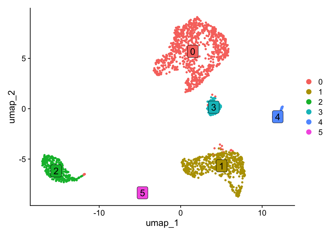
# To improve visualization, we reduced the resolution when identifying cell clusters.
obj <- NormalizeData(obj) %>% FindVariableFeatures() %>% ScaleData() %>%  RunPCA(verbose=FALSE) %>% FindNeighbors(dims = 1:10, verbose=FALSE) %>% FindClusters(resolution = 0.1, verbose=FALSE) %>% RunUMAP(dims=1:10, verbose=FALSE)

Normalizing layer: counts

Finding variable features for layer counts

Centering and scaling data matrix

DimPlot(obj, label=TRUE, label.size = 5, label.box = TRUE)

1. Perform allele-specific gene expression analysis by using SNV anchors

In this vignette, “genetic variant” refers to all alleles at a given locus, including both the reference allele and any alternative alleles. All are annotated and counted by PISA.

var <- ReadPISA("./var")
obj[['var']] <- CreateAssayObject(var[,colnames(obj)], min.cells = 10)
# Switch working assay to 'var'
DefaultAssay(obj) <- "var"

obj <- NormalizeData(obj)

# Skip loading the GTF if you already have it in memory
gtf <- gtf2db("./gencode.v44.annotation.gtf.gz")

[2026-06-15 14:43:53] GTF loading..
[2026-06-15 14:44:23] Load 62700 genes.
[2026-06-15 14:44:23] Load time : 30.139 sec

# Currently the meta information for the variant assay is empty
obj[['var']][[]] %>% head

data frame with 0 columns and 6 rows

obj <- annoVAR(obj, gtf = gtf)

[warnings] Chromosome KI270442.1 not found in GTF, use wrong database? 
[warnings] Chromosome KI270729.1 not found in GTF, use wrong database? 
[warnings] Chromosome GL000205.2 not found in GTF, use wrong database? 
[warnings] Chromosome GL000195.1 not found in GTF, use wrong database? 
[warnings] Chromosome KI270733.1 not found in GTF, use wrong database? 
[warnings] Chromosome GL000219.1 not found in GTF, use wrong database? 
[warnings] Chromosome GL000216.2 not found in GTF, use wrong database? 
[warnings] Chromosome GL000218.1 not found in GTF, use wrong database? 
[warnings] Chromosome KI270713.1 not found in GTF, use wrong database? 

# After annotation, locations are parsed from feature names and overlapping genes are annotated.
obj[['var']][[]] %>% head %>% DT::datatable()

# Select spatially autocorrelated genetic variants
obj <- RunAutoCorr(obj)

For allele-specific expression, we use mode 2 instead of the default mode 1. Mode 2 compares a variant’s expression against other variants at the same locus. Since no separate binding assay is specified, counts at each locus are aggregated, then the test feature is subtracted from the locus total.

obj <- RunSDT(object = obj, bind.name = "locus", mode = 2)

Working on assay var.

Use predefined weight matrix "pca_wm".

Processing 13362 features.

No bind.assay specified, update min.features.per.block to 2.

Processing 4097 binding features.

Use "counts" layer for test features.

Aggregate counts for binding features.

Using 95 threads.

Runtime : 4.861214 secs.

sel.chrs <- c(1:21, "X")
FbtPlot(obj, val = "locus.padj", remove.chr = TRUE, sel.chrs = sel.chrs)

# Randomly pick a pair of features at the same locus
obj[['var']][[]] %>% filter(locus.padj < 1e-10) %>% DT::datatable()

FeaturePlot(obj, features = c("chr10:17237326C>T/+", "chr10:17237326C=/+", "VIM" ), order=TRUE, pt.size = 1, ncol=3)

Warning: Could not find VIM in the default search locations, found in 'RNA'
assay instead

# Zoom into a specific region
FbtPlot(obj, val = "locus.padj", chr="chr10", start = 17225000, end = 17240000, gtf = gtf)

Zoom in chr10 : 17224000-17241000

The T allele of VIM is expressed across most cell groups, while the C allele is primarily restricted to groups 1 and 4.

The spatial dissimilarity test identifies many cases of allele-specific expression. This phenomenon can be driven by gene imprinting, genetic recombination, somatic variants, and other mechanisms. For detailed case studies, see our manuscript.

# Save the Seurat object for further use
saveRDS(obj, file = "glioblastoma5k.rds")

Command(obj)

 [1] "NormalizeData.RNA"        "FindVariableFeatures.RNA"
 [3] "ScaleData.RNA"            "RunPCA.RNA"              
 [5] "FindNeighbors.RNA.pca"    "FindClusters"            
 [7] "RunUMAP.RNA.pca"          "NormalizeData.var"       
 [9] "ParseVarName.var"         "annoVAR.var"             
[11] "RunAutoCorr.var.pca"      "SetAutoCorrFeatures.var" 
[13] "RunSDT.var"              

sessionInfo()

R version 4.5.3 (2026-03-11)
Platform: x86_64-pc-linux-gnu
Running under: Ubuntu 24.04.4 LTS

Matrix products: default
BLAS:   /usr/lib/x86_64-linux-gnu/openblas-pthread/libblas.so.3 
LAPACK: /usr/lib/x86_64-linux-gnu/openblas-pthread/libopenblasp-r0.3.26.so;  LAPACK version 3.12.0

locale:
 [1] LC_CTYPE=C.UTF-8       LC_NUMERIC=C           LC_TIME=C.UTF-8       
 [4] LC_COLLATE=C.UTF-8     LC_MONETARY=C.UTF-8    LC_MESSAGES=C.UTF-8   
 [7] LC_PAPER=C.UTF-8       LC_NAME=C              LC_ADDRESS=C          
[10] LC_TELEPHONE=C         LC_MEASUREMENT=C.UTF-8 LC_IDENTIFICATION=C   

time zone: Etc/UTC
tzcode source: system (glibc)

attached base packages:
[1] stats     graphics  grDevices utils     datasets  methods   base     

other attached packages:
[1] future_1.70.0      Yano_1.5           dplyr_1.2.0        ggplot2_4.0.2     
[5] Seurat_5.4.0       SeuratObject_5.3.0 sp_2.2-1          

loaded via a namespace (and not attached):
  [1] deldir_2.0-4           pbapply_1.7-4          gridExtra_2.3         
  [4] rlang_1.1.7            magrittr_2.0.4         RcppAnnoy_0.0.23      
  [7] otel_0.2.0             spatstat.geom_3.7-3    matrixStats_1.5.0     
 [10] ggridges_0.5.7         compiler_4.5.3         systemfonts_1.3.2     
 [13] png_0.1-9              vctrs_0.7.2            reshape2_1.4.5        
 [16] stringr_1.6.0          pkgconfig_2.0.3        fastmap_1.2.0         
 [19] labeling_0.4.3         promises_1.5.0         rmarkdown_2.30        
 [22] purrr_1.2.1            xfun_0.57              cachem_1.1.0          
 [25] jsonlite_2.0.0         goftest_1.2-3          later_1.4.8           
 [28] spatstat.utils_3.2-2   irlba_2.3.7            parallel_4.5.3        
 [31] cluster_2.1.8.2        R6_2.6.1               ica_1.0-3             
 [34] bslib_0.10.0           stringi_1.8.7          RColorBrewer_1.1-3    
 [37] spatstat.data_3.1-9    reticulate_1.45.0      parallelly_1.46.1     
 [40] spatstat.univar_3.1-7  jquerylib_0.1.4        lmtest_0.9-40         
 [43] scattermore_1.2        Rcpp_1.1.1             knitr_1.51            
 [46] tensor_1.5.1           future.apply_1.20.2    zoo_1.8-15            
 [49] sctransform_0.4.3      httpuv_1.6.17          Matrix_1.7-5          
 [52] splines_4.5.3          igraph_2.2.2           tidyselect_1.2.1      
 [55] viridis_0.6.5          abind_1.4-8            yaml_2.3.12           
 [58] spatstat.random_3.4-5  codetools_0.2-20       miniUI_0.1.2          
 [61] spatstat.explore_3.8-0 listenv_0.10.1         lattice_0.22-9        
 [64] tibble_3.3.1           plyr_1.8.9             withr_3.0.2           
 [67] shiny_1.13.0           S7_0.2.1               ROCR_1.0-12           
 [70] evaluate_1.0.5         Rtsne_0.17             fastDummies_1.7.5     
 [73] survival_3.8-6         polyclip_1.10-7        fitdistrplus_1.2-6    
 [76] pillar_1.11.1          KernSmooth_2.23-26     DT_0.34.0             
 [79] plotly_4.12.0          generics_0.1.4         RcppHNSW_0.6.0        
 [82] scales_1.4.0           gtools_3.9.5           globals_0.19.1        
 [85] xtable_1.8-8           glue_1.8.0             lazyeval_0.2.2        
 [88] tools_4.5.3            data.table_1.18.2.1    RSpectra_0.16-2       
 [91] RANN_2.6.2             dotCall64_1.2          cowplot_1.2.0         
 [94] grid_4.5.3             tidyr_1.3.2            crosstalk_1.2.2       
 [97] nlme_3.1-168           patchwork_1.3.2        cli_3.6.5             
[100] spatstat.sparse_3.1-0  spam_2.11-3            viridisLite_0.4.3     
[103] uwot_0.2.4             gtable_0.3.6           sass_0.4.10           
[106] digest_0.6.39          progressr_0.18.0       ggrepel_0.9.8         
[109] htmlwidgets_1.6.4      farver_2.1.2           htmltools_0.5.9       
[112] lifecycle_1.0.5        httr_1.4.8             mime_0.13             
[115] MASS_7.3-65